Explain Image Classification by SHAP Deep Explainer
Goal
This post aims to introduce how to explain Image Classification (trained by PyTorch) via SHAP Deep Explainer.
Shap is the module to make the black box model interpretable. For example, image classification tasks can be explained by the scores on each pixel on a predicted image, which indicates how much it contributes to the probability positively or negatively.
Reference
Libraries
import torch, torchvision
from torchvision import datasets, transforms
from torch import nn, optim
from torch.nn import functional as F
from torchviz import make_dot
import numpy as np
import shap
import matplotlib.pyplot as plt
%matplotlib inline
Deep Learning Model Preparation
Configuration
batch_size = 128
num_epochs = 2
learning_rate = 0.01
momentum=0.5
device = torch.device('cpu')
Network Definition
class Net(nn.Module):
    def __init__(self):
        super(Net, self).__init__()

        # Convolution Layers
        self.conv_layers = nn.Sequential(
            nn.Conv2d(1, 10, kernel_size=5),
            nn.MaxPool2d(2),
            nn.ReLU(),
            nn.Conv2d(10, 20, kernel_size=5),
            nn.Dropout(),
            nn.MaxPool2d(2),
            nn.ReLU(),
        )

        #
        self.fc_layers = nn.Sequential(
            nn.Linear(320, 50),
            nn.ReLU(),
            nn.Dropout(),
            nn.Linear(50, 10),
            nn.Softmax(dim=1)
        )

    def forward(self, x):
        x = self.conv_layers(x)
        x = x.view(-1, 320)
        x = self.fc_layers(x)
        return x
model = Net()
model
Define Train & Test procedure
The followings are the process in train and test:
-
optimizer.zero_grad()- reset the gradients before update (only training) -
output = model(data)- predict the value based on the current model -
F.nll_loss(output.log(), target)- compute the loss. Here we use negative log likelihood. -
loss.backward()- calculate gradients based on the loss -
optimizer.step()- execute backward propagation to update the weights
def train(model, device, train_loader, optimizer, epoch):
    model.train()
    for batch_idx, (data, target) in enumerate(train_loader):
        data, target = data.to(device), target.to(device)
        optimizer.zero_grad()
        output = model(data)
        loss = F.nll_loss(output.log(), target)
        loss.backward()
        optimizer.step()
        if batch_idx % 100 == 0:
            print('Train Epoch: {} [{}/{} ({:.0f}%)]\tLoss: {:.6f}'.format(
                epoch, batch_idx * len(data), len(train_loader.dataset),
                100. * batch_idx / len(train_loader), loss.item()))


def test(model, device, test_loader):
    model.eval()
    test_loss = 0
    correct = 0
    with torch.no_grad():
        for data, target in test_loader:
            data, target = data.to(device), target.to(device)
            output = model(data)

            # sum up batch loss
            test_loss += F.nll_loss(output.log(),
                                    target).item()

            # get the index of the max log-probability
            pred = output.max(1, keepdim=True)[1]
            correct += pred.eq(target.view_as(pred)).sum().item()

    test_loss /= len(test_loader.dataset)
    print(
        '\nTest set: Average loss: {:.4f}, Accuracy: {}/{} ({:.0f}%)\n'.format(
            test_loss, correct, len(test_loader.dataset),
            100. * correct / len(test_loader.dataset)))
Prepare data loader
train_loader/test_loader is the iterator to generate a collection of images.
train_loader = torch.utils.data.DataLoader(datasets.MNIST(
    'mnist_data',
    train=True,
    download=True,
    transform=transforms.Compose([transforms.ToTensor()])),
    batch_size=batch_size,
    shuffle=True)

test_loader = torch.utils.data.DataLoader(datasets.MNIST(
    'mnist_data',
    train=False,
    transform=transforms.Compose([transforms.ToTensor()])),
    batch_size=batch_size,
    shuffle=True)
batch = next(iter(train_loader))
images, labels = batch
plt.imshow(images[:1][0][0].numpy());
plt.title(f'Images for {str(labels[:1][0].numpy())}');

Execute training and testing
# Instantiate the model and optimizer
model = Net().to(device)
optimizer = optim.SGD(model.parameters(), lr=learning_rate, momentum=momentum)

for epoch in range(1, num_epochs + 1):
    train(model, device, train_loader, optimizer, epoch)
    test(model, device, test_loader)
Create Deep Explainer
Load some images for explainer
# since shuffle=True, this is a random sample of test data
batch = next(iter(test_loader))
images, _ = batch
images.size()
Instanciate Deep Explainer with background images (100 imagesm)
background = images[:100]
e = shap.DeepExplainer(model, background)
e
Explain the test images
n_test_images = 10
test_images = images[100:100+n_test_images]
shap_values = e.shap_values(test_images)
# rehspae the shap value array and test image array for visualization
shap_numpy = [np.swapaxes(np.swapaxes(s, 1, -1), 1, 2) for s in shap_values]
test_numpy = np.swapaxes(np.swapaxes(test_images.numpy(), 1, -1), 1, 2)
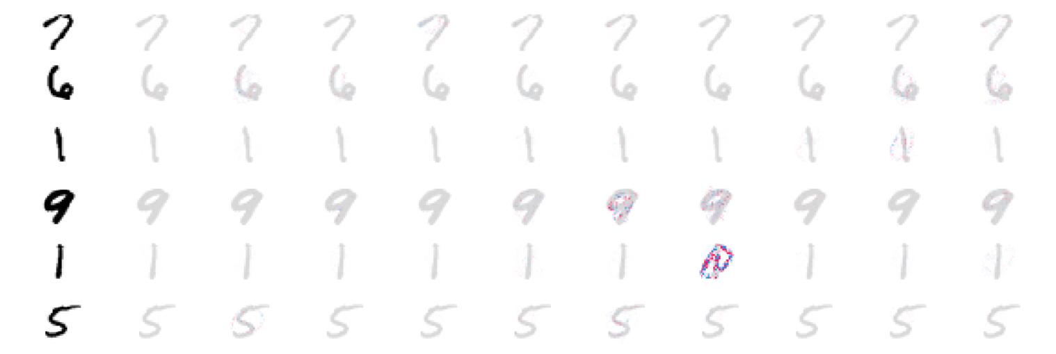
Visualize SHAP value for test images
The shap value that indicate the score for each class are shown as below. The rows indicate the test images and the columns are the classes from 0 to 9 going left to right.
Note that the obtained score as below does not make sense against the original example notebook. For example, 5th prediction for "1" has a lot of positive value on "6"
# plot the feature attributions
shap.image_plot(shap_numpy, -test_numpy)

Comments
Comments powered by Disqus