Posts about pandas

One-Hot Encode Nominal Categorical Features

Goal

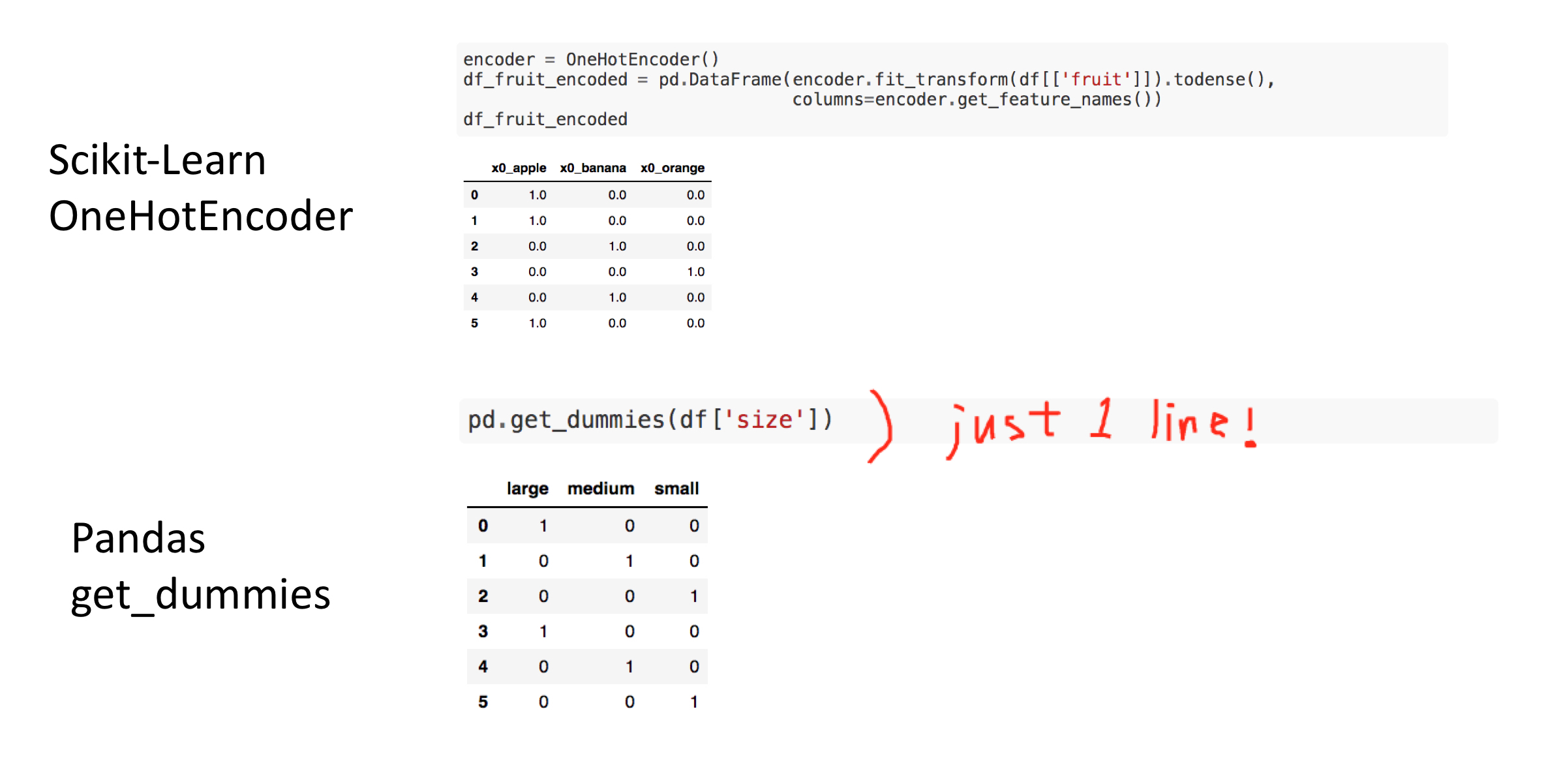
This post aims to introduce how to create one-hot-encoded features for categorical variables. In this post, two ways of creating one hot encoded features: OneHotEncoder in scikit-learn and get_dummies in pandas.

Peronally, I like get_dummies in pandas since pandas takes care of columns names, type of data and therefore, it looks cleaner and simpler with less code.

image

Reference

Calculate The Average, Variance, And Standard Deviation

Goal

This post aims to introduce how to calculate the average, variance and standard deviation of matrix using pandas.

Libraries

In [2]:
import pandas as pd
import numpy as np

Create a matrix

In [13]:
n = 1000
df = pd.DataFrame({'rand': np.random.rand(n),
                   'randint': np.random.randint(low=0, high=100, size=n),
                   'randn': np.random.randn(n),
                   'random_sample': np.random.random_sample(size=n),
                   'binomial': np.random.binomial(n=1, p=.5, size=n),
                   'beta': np.random.beta(a=1, b=1, size=n),
                   })
df.head()
Out[13]:
rand randint randn random_sample binomial beta
0 0.689690 59 0.416245 0.607567 1 0.532052
1 0.288356 2 0.092351 0.311634 0 0.192651
2 0.173002 50 -0.626691 0.920702 0 0.342812
3 0.953088 17 -0.149677 0.316060 1 0.792191
4 0.693120 94 0.264678 0.060313 1 0.059370

Calculate average, variance, and standard deviation

Calculate by each function

In [16]:
df.mean()
Out[16]:
rand              0.497015
randint          49.224000
randn            -0.054651
random_sample     0.504412
binomial          0.490000
beta              0.508469
dtype: float64
In [15]:
df.var()
Out[15]:
rand               0.083301
randint          791.485309
randn              1.033378
random_sample      0.081552
binomial           0.250150
beta               0.083489
dtype: float64
In [17]:
df.std()
Out[17]:
rand              0.288619
randint          28.133349
randn             1.016552
random_sample     0.285573
binomial          0.500150
beta              0.288944
dtype: float64

Calculate using describe

In [18]:
df.describe()
Out[18]:
rand randint randn random_sample binomial beta
count 1000.000000 1000.000000 1000.000000 1000.000000 1000.00000 1000.000000
mean 0.497015 49.224000 -0.054651 0.504412 0.49000 0.508469
std 0.288619 28.133349 1.016552 0.285573 0.50015 0.288944
min 0.000525 0.000000 -3.405606 0.001359 0.00000 0.000373
25% 0.241000 25.000000 -0.741640 0.264121 0.00000 0.256070
50% 0.497571 48.000000 -0.074852 0.505738 0.00000 0.523674
75% 0.742702 73.000000 0.602928 0.743445 1.00000 0.758901
max 0.999275 99.000000 3.861652 0.995010 1.00000 0.999007

Select Date And Time Ranges

Goal

This post aims to introduce how to select a subset of the pandas dataframe by selecting a date range.

Libraries

In [2]:
import pandas as pd
import numpy as np

Create a dataframe

In [18]:
date_ranges = pd.date_range('20190101', '20191231', freq='d')
df_rand = pd.DataFrame({'date': date_ranges, 
                       'value': np.random.random(date_ranges.shape[0])})
df_rand.head()
Out[18]:
date value
0 2019-01-01 0.332090
1 2019-01-02 0.690167
2 2019-01-03 0.237744
3 2019-01-04 0.060678
4 2019-01-05 0.572691

Select a range using .between

In [19]:
df_rand.loc[df_rand.date.between('20190201', '20190211'),:]
Out[19]:
date value
31 2019-02-01 0.449901
32 2019-02-02 0.803429
33 2019-02-03 0.299074
34 2019-02-04 0.630970
35 2019-02-05 0.294973
36 2019-02-06 0.510857
37 2019-02-07 0.345567
38 2019-02-08 0.877957
39 2019-02-09 0.990186
40 2019-02-10 0.000186
41 2019-02-11 0.378379

Convert Strings To Dates

Goal

This post aims to introduce how to convert strings to dates using pandas

Libraries

In [1]:
import pandas as pd

Date in string

In [3]:
df_date = pd.DataFrame({'date':['20190101', '20190102', '20190105'], 
                       'temperature': [23.5, 32, 25]})
df_date
Out[3]:
date temperature
0 20190101 23.5
1 20190102 32.0
2 20190105 25.0

Convert strings to date format

In [4]:
pd.to_datetime(df_date['date'])
Out[4]:
0   2019-01-01
1   2019-01-02
2   2019-01-05
Name: date, dtype: datetime64[ns]

Describe An Array

Goal

This post aims to describe an array using pandas. As an example, Boston Housing Data is used in this post.

Reference

Libraries

In [13]:
import pandas as pd
from sklearn.datasets import load_boston
%matplotlib inline

Create an array

In [4]:
boston = load_boston()
df_boston = pd.DataFrame(boston['data'], columns=boston['feature_names'])
df_boston.head()
Out[4]:
CRIM ZN INDUS CHAS NOX RM AGE DIS RAD TAX PTRATIO B LSTAT
0 0.00632 18.0 2.31 0.0 0.538 6.575 65.2 4.0900 1.0 296.0 15.3 396.90 4.98
1 0.02731 0.0 7.07 0.0 0.469 6.421 78.9 4.9671 2.0 242.0 17.8 396.90 9.14
2 0.02729 0.0 7.07 0.0 0.469 7.185 61.1 4.9671 2.0 242.0 17.8 392.83 4.03
3 0.03237 0.0 2.18 0.0 0.458 6.998 45.8 6.0622 3.0 222.0 18.7 394.63 2.94
4 0.06905 0.0 2.18 0.0 0.458 7.147 54.2 6.0622 3.0 222.0 18.7 396.90 5.33

Describe numerical values

pandas DataFrame has a method, called describe, which shows basic statistics based on the data types for each columns

In [5]:
df_boston.describe()
Out[5]:
CRIM ZN INDUS CHAS NOX RM AGE DIS RAD TAX PTRATIO B LSTAT
count 506.000000 506.000000 506.000000 506.000000 506.000000 506.000000 506.000000 506.000000 506.000000 506.000000 506.000000 506.000000 506.000000
mean 3.613524 11.363636 11.136779 0.069170 0.554695 6.284634 68.574901 3.795043 9.549407 408.237154 18.455534 356.674032 12.653063
std 8.601545 23.322453 6.860353 0.253994 0.115878 0.702617 28.148861 2.105710 8.707259 168.537116 2.164946 91.294864 7.141062
min 0.006320 0.000000 0.460000 0.000000 0.385000 3.561000 2.900000 1.129600 1.000000 187.000000 12.600000 0.320000 1.730000
25% 0.082045 0.000000 5.190000 0.000000 0.449000 5.885500 45.025000 2.100175 4.000000 279.000000 17.400000 375.377500 6.950000
50% 0.256510 0.000000 9.690000 0.000000 0.538000 6.208500 77.500000 3.207450 5.000000 330.000000 19.050000 391.440000 11.360000
75% 3.677083 12.500000 18.100000 0.000000 0.624000 6.623500 94.075000 5.188425 24.000000 666.000000 20.200000 396.225000 16.955000
max 88.976200 100.000000 27.740000 1.000000 0.871000 8.780000 100.000000 12.126500 24.000000 711.000000 22.000000 396.900000 37.970000

Adding Or Substracting Time

Goal

This post aims to add or subtract time from date column using pandas:

  • Pandas

Reference:

  • Chris Albon's blog (I look at his post's title and wrote my own contents to deepen my understanding about the topic.)

Library

In [1]:
import pandas as pd

Create date columns using date_range

In [2]:
date_rng = pd.date_range(start='20160101', end='20190101', freq='m', closed='left')
date_rng
Out[2]:
DatetimeIndex(['2016-01-31', '2016-02-29', '2016-03-31', '2016-04-30',
               '2016-05-31', '2016-06-30', '2016-07-31', '2016-08-31',
               '2016-09-30', '2016-10-31', '2016-11-30', '2016-12-31',
               '2017-01-31', '2017-02-28', '2017-03-31', '2017-04-30',
               '2017-05-31', '2017-06-30', '2017-07-31', '2017-08-31',
               '2017-09-30', '2017-10-31', '2017-11-30', '2017-12-31',
               '2018-01-31', '2018-02-28', '2018-03-31', '2018-04-30',
               '2018-05-31', '2018-06-30', '2018-07-31', '2018-08-31',
               '2018-09-30', '2018-10-31', '2018-11-30', '2018-12-31'],
              dtype='datetime64[ns]', freq='M')