Posts about Deep Learning

Explain Image Classification by SHAP Deep Explainer

Goal

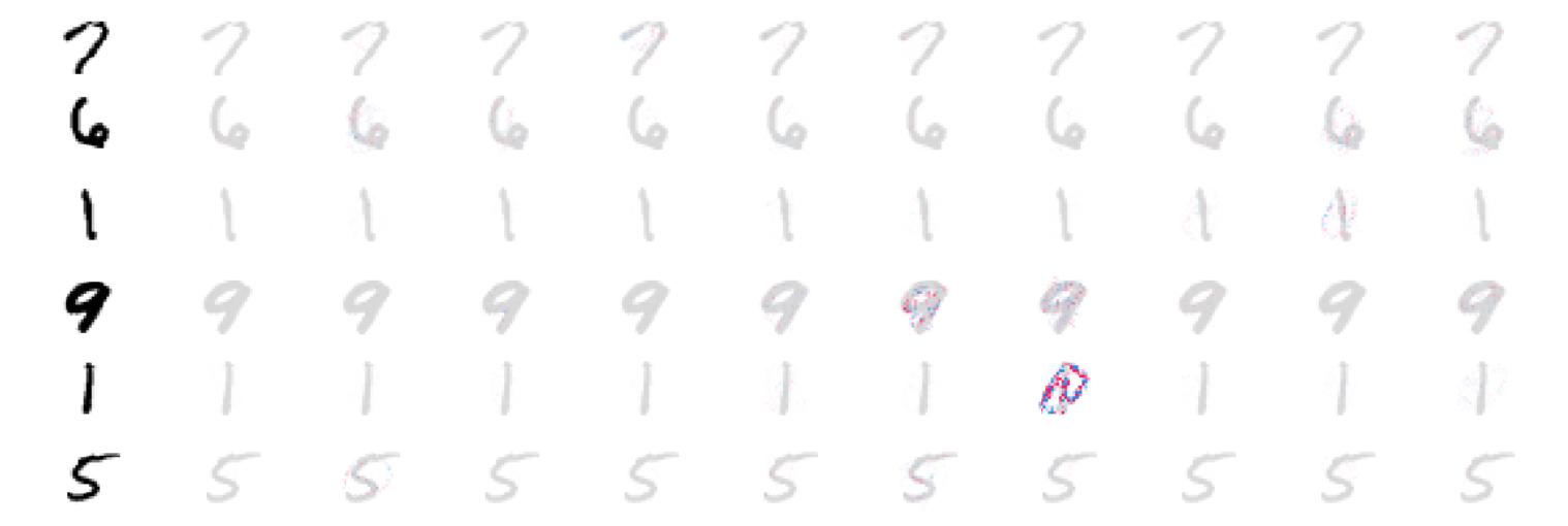
This post aims to introduce how to explain Image Classification (trained by PyTorch) via SHAP Deep Explainer.

Shap is the module to make the black box model interpretable. For example, image classification tasks can be explained by the scores on each pixel on a predicted image, which indicates how much it contributes to the probability positively or negatively.

image

Reference

Loss Functions in Deep Learning with PyTorch

Goal

This post aims to compare loss functions in deep learning with PyTorch.

The following loss functions are covered in this post:

  • Mean Absolute Error (L1 Loss)
  • Mean Square Error (L2 Loss)
  • Binary Cross Entropy (BCE)
  • Kullback-Leibler divergence (KL divergence)

image

Reference

How to Develop a 1D Generative Adversarial Network From Scratch in PyTorch (Part 1)

Goal

This post is inspired by the blog "Machine Learning Mastery - How to Develop a 1D Generative Adversarial Network From Scratch in Keras" written by Jason Brownlee, PhD. But to learn step-by-step, I will describe the same concept with PyTorch.

This post will cover the followings:

Part 1:

  • Select a One-Dimensional Function
  • Define a Discriminator Model

Reference

Libraries

In [33]:
import pandas as pd
import numpy as np
import matplotlib.pyplot as plt
%matplotlib inline

# PyTorch
import torch
from torch import nn
from torch import optim
from torchviz import make_dot

Create a target 1-D function

In [3]:
def f(x):
    return x **2
In [17]:
n = 100
sigma = 10
x = sigma * (np.random.random(size=n) - 0.5)
plt.plot(x, f(x), '.');
plt.title('Target function $f(x)$');
plt.xlabel('randomly sampled x');
plt.ylabel('$f(x)$');

Define a Discriminator Model

The definition of a discriminator model is that it will classify the input data into real or fake

In [35]:
# Build a feed-forward network
model = nn.Sequential(nn.Linear(2, 25),
                      nn.ReLU(),
                      nn.Sigmoid()
                     )

# Loss
criterion = nn.CrossEntropyLoss()

# Optimizer
optimizer = optim.Adam(model.parameters(), lr=0.001)
In [36]:
# Visualize this neural network
x = torch.zeros(0, 2, dtype=torch.float, requires_grad=False)
out = model(x)
make_dot(out)
Out[36]:
%3 4870964168 SigmoidBackward4870966520 ThresholdBackward04870966520->4870964168 4870966072 AddmmBackward4870966072->4870966520 4870966296 (25)4870966296->4870966072 4870966240 TBackward4870966240->4870966072 4940643408 (25, 2)4940643408->4870966240

Create real and fake samples

In [79]:
def generate_samples(size=100, label='real'):
    """Generate samples with real or fake label
    """
    x = np.random.randn(size, 1)
    x2 = f(x)
    
    y = np.ones((size, 1)) * (label == 'real')
    return np.hstack([x, x2]), y
    
In [80]:
X, y = generate_samples()
In [82]:
x[:5]
Out[82]:
array([[ 1.2483621 ,  1.55840793],
       [ 0.57980381,  0.33617245],
       [-0.06718955,  0.00451444],
       [-1.95352245,  3.81624995],
       [-1.14922801,  1.32072501]])
In [83]:
y[:5]
Out[83]:
array([[1.],
       [1.],
       [1.],
       [1.],
       [1.]])

Train the image classifier using PyTorch

Goal

This post aims to introduce how to train the image classifier for MNIST dataset using PyTorch

image

Reference

Libraries

In [8]:
import pandas as pd
import numpy as np
import matplotlib.pyplot as plt
%matplotlib inline

# Dataset
from sklearn.datasets import load_digits

# PyTorch
import torch 
import torchvision
import torchvision.transforms as transforms

import torch.nn as nn
import torch.nn.functional as F
import torch.optim as optim

Functions

In [32]:
def imshow(img):
    img = img / 2 + 0.5 # unnormalize
    npimg = img.numpy()
    plt.imshow(np.transpose(npimg, (1, 2, 0)))
    plt.axis('off')
    plt.show()

Load MNIST dataset

When downloading the image dataset, we also need to define transform function that apply pixel normalization from [0, 1] to [-1, +1]

In [50]:
transform = transforms.Compose(
    [transforms.ToTensor(),
     transforms.Normalize((0.5, ), (0.5, ))])

trainset = torchvision.datasets.MNIST(root='~/data', 
                                        train=True,
                                        download=True,
                                        transform=transform)

testset = torchvision.datasets.MNIST(root='~/data', 
                                        train=False, 
                                        download=True, 
                                        transform=transform)
9920512it [00:28, 1582029.76it/s]                             

1654784it [00:23, 573182.07it/s]                             

Create a dataloader

In [13]:
trainloader = torch.utils.data.DataLoader(trainset,
                                          batch_size=100,
                                          shuffle=True,
                                          num_workers=2)
In [14]:
testloader = torch.utils.data.DataLoader(testset,
                                         batch_size=100,
                                         shuffle=False,
                                         num_workers=2)

Define a model

In [6]:
class Net(nn.Module):
    def __init__(self):
        super(Net, self).__init__()
        self.conv1 = nn.Conv2d(1, 32, 3)  # 28x28x32 -> 26x26x32
        self.conv2 = nn.Conv2d(32, 64, 3)  # 26x26x64 -> 24x24x64
        self.pool = nn.MaxPool2d(2, 2)  # 24x24x64 -> 12x12x64
        self.dropout1 = nn.Dropout2d()
        self.fc1 = nn.Linear(12 * 12 * 64, 128)
        self.dropout2 = nn.Dropout2d()
        self.fc2 = nn.Linear(128, 10)

    def forward(self, x):
        x = F.relu(self.conv1(x))
        x = self.pool(F.relu(self.conv2(x)))
        x = self.dropout1(x)
        x = x.view(-1, 12 * 12 * 64)
        x = F.relu(self.fc1(x))
        x = self.dropout2(x)
        x = self.fc2(x)
        return x

Create a loss function and optimizer

In [10]:
model = Net()
criterion = nn.CrossEntropyLoss()
optimizer = optim.SGD(model.parameters(), lr=0.001, momentum=0.9)

Training a model

In [22]:
epochs = 5
for epoch in range(epochs):
    running_loss = 0.0
    for i, (inputs, labels) in enumerate(trainloader, 0):
        # zero the parameter gradients
        optimizer.zero_grad()

        # forward + backward + optimize
        outputs = model(inputs)
        loss = criterion(outputs, labels)
        loss.backward()
        optimizer.step()

        # print statistics
        running_loss += loss.item()
        if i % 100 == 99:
            print(f'[{epoch + 1}, {i+1}] loss: {running_loss / 100:.2}')
            running_loss = 0.0

print('Finished Training')
[1, 100] loss: 1.5
[1, 200] loss: 0.82
[1, 300] loss: 0.63
[1, 400] loss: 0.55
[1, 500] loss: 0.5
[1, 600] loss: 0.46
[2, 100] loss: 0.42
[2, 200] loss: 0.4
[2, 300] loss: 0.38
[2, 400] loss: 0.38
[2, 500] loss: 0.34
[2, 600] loss: 0.34
[3, 100] loss: 0.31
[3, 200] loss: 0.31
[3, 300] loss: 0.29
[3, 400] loss: 0.28
[3, 500] loss: 0.28
[3, 600] loss: 0.26
[4, 100] loss: 0.24
[4, 200] loss: 0.24
[4, 300] loss: 0.24
[4, 400] loss: 0.23
[4, 500] loss: 0.23
[4, 600] loss: 0.22
[5, 100] loss: 0.2
[5, 200] loss: 0.21
[5, 300] loss: 0.2
[5, 400] loss: 0.19
[5, 500] loss: 0.19
[5, 600] loss: 0.19
Finished Training

Test

In [37]:
dataiter = iter(testloader)
images, labels = dataiter.next()
outputs = model(images)
_, predicted = torch.max(outputs, 1)
In [48]:
n_test = 10
df_result = pd.DataFrame({
    'Ground Truth': labels[:n_test],
    'Predicted label': predicted[:n_test]})
display(df_result.T)
imshow(torchvision.utils.make_grid(images[:n_test, :, :, :], nrow=n_test))
0 1 2 3 4 5 6 7 8 9
Ground Truth 7 2 1 0 4 1 4 9 5 9
Predicted label 7 2 1 0 4 1 4 9 6 9

Style Transfer using Pytorch (Part 4)

Libraries

In [12]:
import pandas as pd
import copy

# Torch & Tensorflow
import torch
import torch.nn as nn
import torch.nn.functional as F
import torchvision
import tensorflow as tf

# Visualization
from torchviz import make_dot
from PIL import Image
import matplotlib.pyplot as plt
%matplotlib inline

import warnings

Configuration

In [2]:
device = torch.device("cuda" if torch.cuda.is_available() else "cpu")

Functions

The functions covered by the previous posts (Part 1, Part 2, Part 3) are as follows.

Functions from Part 1 - image loader

In [46]:
# desired size of the output image
imsize = (512, 512) if torch.cuda.is_available() else (128, 128)  # use small size if no gpu

loader = torchvision.transforms.Compose([
    torchvision.transforms.Resize(imsize),  # scale imported image
    torchvision.transforms.ToTensor()])  # transform it into a torch tensor

def image_loader(image_name):
    image = Image.open(image_name)

    # fake batch dimension required to fit network's input dimensions
    image = loader(image).unsqueeze(0)
    return image.to(device, torch.float)
In [5]:
unloader = torchvision.transforms.ToPILImage() 

def imshow_tensor(tensor, ax=None):
    image = tensor.cpu().clone()  # we clone the tensor to not do changes on it
    image = image.squeeze(0)      # remove the fake batch dimension

    image = unloader(image)
    if ax:
        ax.imshow(image)
    else:
        plt.imshow(image)

Functions from Part 2 - loss functions

In [6]:
class ContentLoss(nn.Module):

    def __init__(self, target,):
        super(ContentLoss, self).__init__()
        self.target = target.detach()

    def forward(self, input):
        self.loss = F.mse_loss(input, self.target)
        return input
    
def gram_matrix(input):
    # Get the size of tensor
    # a: batch size
    # b: number of feature maps
    # c, d: the dimension of a feature map
    a, b, c, d = input.size() 
    
    # Reshape the feature 
    features = input.view(a * b, c * d)

    # Multiplication
    G = torch.mm(features, features.t())  
    
    # Normalize 
    G_norm = G.div(a * b * c * d)
    return G_norm

class StyleLoss(nn.Module):

    def __init__(self, target_feature):
        super(StyleLoss, self).__init__()
        self.target = gram_matrix(target_feature).detach()

    def forward(self, input):
        G = gram_matrix(input)
        self.loss = F.mse_loss(G, self.target)
        return input

Functions from Part 3 - modeling

Normalization

In [7]:
cnn_normalization_mean = torch.tensor([0.485, 0.456, 0.406]).to(device)
cnn_normalization_std = torch.tensor([0.229, 0.224, 0.225]).to(device)

# create a module to normalize input image so we can easily put it in a
# nn.Sequential
class Normalization(nn.Module):
    def __init__(self, mean, std):
        super(Normalization, self).__init__()
        # .view the mean and std to make them [C x 1 x 1] so that they can
        # directly work with image Tensor of shape [B x C x H x W].
        # B is batch size. C is number of channels. H is height and W is width.
        self.mean = torch.tensor(mean).view(-1, 1, 1)
        self.std = torch.tensor(std).view(-1, 1, 1)

    def forward(self, img):
        # normalize img
        return (img - self.mean) / self.std

Create a sequential model for style transfer

In [8]:
# desired depth layers to compute style/content losses :
content_layers_default = ['conv_4']
style_layers_default = ['conv_1', 'conv_2', 'conv_3', 'conv_4', 'conv_5']

def get_style_model_and_losses(cnn, normalization_mean, normalization_std,
                               style_img, content_img,
                               content_layers=content_layers_default,
                               style_layers=style_layers_default):
    cnn = copy.deepcopy(cnn)

    # normalization module
    normalization = Normalization(normalization_mean, normalization_std).to(device)

    # just in order to have an iterable access to or list of content/syle
    # losses
    content_losses = []
    style_losses = []

    # assuming that cnn is a nn.Sequential, so we make a new nn.Sequential
    # to put in modules that are supposed to be activated sequentially
    model = nn.Sequential(normalization)

    i = 0  # increment every time we see a conv
    for n_child, layer in enumerate(cnn.children()):
#         print()
#         print(f"n_child: {n_child}")
        if isinstance(layer, nn.Conv2d):
            i += 1
            name = 'conv_{}'.format(i)
        elif isinstance(layer, nn.ReLU):
            name = 'relu_{}'.format(i)
            # The in-place version doesn't play very nicely with the ContentLoss
            # and StyleLoss we insert below. So we replace with out-of-place
            # ones here.
            layer = nn.ReLU(inplace=False)
        elif isinstance(layer, nn.MaxPool2d):
            name = 'pool_{}'.format(i)
        elif isinstance(layer, nn.BatchNorm2d):
            name = 'bn_{}'.format(i)
        else:
            raise RuntimeError('Unrecognized layer: {}'.format(layer.__class__.__name__))

        model.add_module(name, layer)
#         print(f'Name: {name}')
        if name in content_layers:
#             print(f'Add content loss {i}')
            # add content loss:
            target = model(content_img).detach()
            content_loss = ContentLoss(target)
            model.add_module("content_loss_{}".format(i), content_loss)
            content_losses.append(content_loss)

        if name in style_layers:
#             print(f'Add style loss {i}')
            # add style loss:
            target_feature = model(style_img).detach()
            style_loss = StyleLoss(target_feature)
            model.add_module("style_loss_{}".format(i), style_loss)
            style_losses.append(style_loss)

    # now we trim off the layers after the last content and style losses
    for i in range(len(model) - 1, -1, -1):
        if isinstance(model[i], ContentLoss) or isinstance(model[i], StyleLoss):
            break

    model = model[:(i + 1)]

    return model, style_losses, content_losses

Load images

In [65]:
d_path = {}
d_path['content'] = tf.keras.utils.get_file('turtle.jpg','https://storage.googleapis.com/download.tensorflow.org/example_images/Green_Sea_Turtle_grazing_seagrass.jpg')
d_path['style'] = tf.keras.utils.get_file('kandinsky.jpg','https://storage.googleapis.com/download.tensorflow.org/example_images/Vassily_Kandinsky%2C_1913_-_Composition_7.jpg')
In [142]:
style_img = image_loader(d_path['style'])[:, :, :, :170]
content_img = image_loader(d_path['content'])[:, :, :, :170]
input_img = content_img.clone()

assert style_img.size() == content_img.size(), \
    "we need to import style and content images of the same size"

Modeling

In [80]:
# Obtain the model for style transfer
# with warnings.catch_warnings():
warnings.filterwarnings("ignore")
cnn = torchvision.models.vgg19(pretrained=True).features.to(device).eval()
model, style_losses, content_losses = get_style_model_and_losses(cnn, cnn_normalization_mean, cnn_normalization_std, style_img, content_img)

Executing a neural transfer

Gradient Decent

L-BFGS stands for Limited-memory Broyden–Fletcher–Goldfarb–Shanno according to wiki - Limited-memory_BFGS, which is one of the optimization algorithm using limited amount of memory.

In [81]:
def get_input_optimizer(input_img):
    # this line to show that input is a parameter that requires a gradient
    optimizer = torch.optim.LBFGS([input_img.requires_grad_()])
    return optimizer

optimizer = get_input_optimizer(input_img)

Execution

The execution steps in the function get_style_model_and_losses in NEURAL TRANSFER USING PYTORCH are as follows:

  1. Initialization
  2. Parameter
  3. Define closure function to re-evaluate the model to execute the followings:
    • masking images between 0 and 1 by .clamp method
    • reset gradient by zero_grad method
    • reset the error score for style and content
    • compute the style and content loss in each inserted layer
    • compute the sum of the losses for style and content
    • multiply the weight for style and content to manipulate the style transfer balance by input argument
    • execute error back propagation
  4. Execute the steps by gradient descent optimizer
In [120]:
# Parameters
num_steps = 10
style_weight=5000
content_weight=1
input_img = content_img[:, :, :, :170].clone()
d_images = {}

print('Building the style transfer model..')
model, style_losses, content_losses = get_style_model_and_losses(cnn,
    cnn_normalization_mean, cnn_normalization_std, style_img, content_img)
optimizer = get_input_optimizer(input_img)

# Execution
run = [0]
while run[0] <= num_steps:

    def closure():
        # correct the values of updated input image
        input_img.data.clamp_(0, 1)

        optimizer.zero_grad()
        model(input_img)
        style_score = 0
        content_score = 0

        for sl in style_losses:
            style_score += sl.loss
        for cl in content_losses:
            content_score += cl.loss

        style_score *= style_weight
        content_score *= content_weight

        loss = style_score + content_score
        loss.backward()

        run[0] += 1
        if run[0] % 2 == 0:
            print("run {}:".format(run))
            print('Style Loss : {:4f} Content Loss: {:4f}'.format(
                style_score.item(), content_score.item()))
            input_img.data.clamp_(0, 1)
            d_images[run[0]] = input_img
            print()

        return style_score + content_score

    optimizer.step(closure)

    # a last correction...
    input_img.data.clamp_(0, 1)
Building the style transfer model..
run [2]:
Style Loss : 1004.939392 Content Loss: 0.000014

run [4]:
Style Loss : 644.263489 Content Loss: 24.647982

run [6]:
Style Loss : 558.792542 Content Loss: 55.995193

run [8]:
Style Loss : 241.166168 Content Loss: 41.970711

run [10]:
Style Loss : 143.137131 Content Loss: 51.402943

run [12]:
Style Loss : 88.965408 Content Loss: 55.758999

run [14]:
Style Loss : 57.654659 Content Loss: 60.926662

run [16]:
Style Loss : 48.282879 Content Loss: 57.995407

run [18]:
Style Loss : 36.090813 Content Loss: 58.100056

run [20]:
Style Loss : 26.983953 Content Loss: 56.346275

In [141]:
fig, axes = plt.subplots(1, 3, figsize=(16, 8))
d_img = {"Content": content_img,
         "Style": style_img,
         "Output": input_img}
for i, key in enumerate(d_img.keys()):
    imshow_tensor(d_img[key], ax=axes[i])
    axes[i].set_title(f"{key} Image")
    axes[i].axis('off')

Visualize the process of style transfer

This is not yet obvious to see the processes of style transfer. It seems run 2 already finish most of the transfer processes. This needs to be investigated later.

In [128]:
fig, axes = plt.subplots(int(len(d_images)/2), 2, figsize=(16, 20))
for i, key in enumerate(d_images.keys()):
    imshow_tensor(d_images[key], ax=axes[i//2][i%2])
    axes[i//2][i%2].set_title("run {}:".format(key))
    axes[i//2][i%2].axis('off')

Style Transfer using Pytorch (Part 3)

Style Transfer using Pytorch (Part 2)

Libraries

In [76]:
import pandas as pd

# Torch & Tensorflow
import torch
import torch.nn as nn
import torch.nn.functional as F
import tensorflow as tf

# Visualization
from PIL import Image
import matplotlib.pyplot as plt
%matplotlib inline

Loss Functions

Content loss

Content loss is calculated using MSE (Mean Square Error) between the content images and the output image:

$$MSE = \frac{1}{n} \sum^{n}_{i=1} (Y_{content} - Y_{output})^2$$