Posts about Machine Learning (old posts, page 2)

Remove Punctuation

Goal

This post aims to introduce how to remove punctuation using string.

Reference

Libraries

In [9]:
import string

Create a document

In [10]:
documents = ["this isn't a sample.", 
            'this is another example.' ,
            'this" also appears in the second example.'
            'Is this an example?']

documents
Out[10]:
["this isn't a sample.",
 'this is another example.',
 'this" also appears in the second example.Is this an example?']

Remove Punctuation

In [11]:
table = str.maketrans('', '', string.punctuation)
doc_removed_punctuation = [w.translate(table) for w in documents]
doc_removed_punctuation
Out[11]:
['this isnt a sample',
 'this is another example',
 'this also appears in the second exampleIs this an example']

Bag Of Words

Goal

This post aims to introduce Bag of words which can be used as features for each document or images.

Simply, bag of words are frequency of word with associated index for each word.

Libaries

In [17]:
import pandas as pd
from sklearn.feature_extraction.text import CountVectorizer
from sklearn.feature_extraction.text import TfidfTransformer

Create a document

In [18]:
documents = ['this is a sample.', 
            'this is another example. "this" also appears in the second example.']

documents
Out[18]:
['this is a sample.',
 'this is another example. "this" also appears in the second example.']

Create a count vector

In [19]:
count_vect = CountVectorizer()
word_counts = count_vect.fit_transform(documents)

df_word_counts = pd.DataFrame(word_counts.todense(), columns=count_vect.get_feature_names())
df_word_counts
Out[19]:
also another appears example in is sample second the this
0 0 0 0 0 0 1 1 0 0 1
1 1 1 1 2 1 1 0 1 1 2

Create a frequency vector

In [20]:
tf_transformer = TfidfTransformer(use_idf=False).fit(df_word_counts)
word_freq = tf_transformer.transform(df_word_counts)
df_word_freq = pd.DataFrame(word_freq.todense(), columns=count_vect.get_feature_names())
df_word_freq
Out[20]:
also another appears example in is sample second the this
0 0.000000 0.000000 0.000000 0.000000 0.000000 0.577350 0.57735 0.000000 0.000000 0.577350
1 0.258199 0.258199 0.258199 0.516398 0.258199 0.258199 0.00000 0.258199 0.258199 0.516398

Term Frequency Inverse Document Frequency

Goal

This post aims to introduce term frequency-inverse document frequency as known as TF-IDF, which indicates the importance of the words in a document considering the frequency of them across multiple documents and used for feature creation.

Term Frequency (TF)

Term Frequency can be computed as the number of occurrence of the word $n_{word}$ divided by the total number of words in a document $N_{word}$.

\begin{equation*} TF = \frac{n_{word}}{N_{word}} \end{equation*}

Document Frequency (DF)

Document Frequency can be computed as the number of documents containing the word $n_{doc}$ divided by the number of documents $N_{doc}$.

\begin{equation*} DF = \frac{n_{doc}}{N_{doc}} \end{equation*}

Inverse Document Frequency (IDF)

The inverse document frequency is the inverse of DF.

\begin{equation*} IDF = \frac{N_{doc}}{n_{doc}} \end{equation*}

Practically, to avoid the explosion of IDF and dividing by zero, IDF can be computed by log format with adding 1 to denominator as below.

\begin{equation*} IDF = log(\frac{N_{doc}}{n_{doc}+1}) \end{equation*}

Reference

Libraries

In [18]:
import pandas as pd
from sklearn.feature_extraction.text import TfidfVectorizer

Create a document

In [36]:
documents = ['this is a sample.', 
            'this is another example. "this" also appears in the second example.']

documents
Out[36]:
['this is a sample.',
 'this is another example. "this" also appears in the second example.']

Apply TF-IDF vectorizer

Now applying TF-IDF to each sentence, we will obtain the feature vector for each document accordingly.

In [37]:
vectorizer = TfidfVectorizer()
X = vectorizer.fit_transform(documents)
df_tfidf = pd.DataFrame(X.todense(), columns=vectorizer.get_feature_names())
df_tfidf
Out[37]:
also another appears example in is sample second the this
0 0.00000 0.00000 0.00000 0.00000 0.00000 0.501549 0.704909 0.00000 0.00000 0.501549
1 0.28249 0.28249 0.28249 0.56498 0.28249 0.200994 0.000000 0.28249 0.28249 0.401988
In [38]:
# The highest TF-IDF for each document
df_tfidf.idxmax(axis=1)
Out[38]:
0     sample
1    example
dtype: object
In [39]:
# TF-IDF is zero if the word does not appear in a document
df_tfidf==0
Out[39]:
also another appears example in is sample second the this
0 True True True True True False False True True False
1 False False False False False False True False False False

Survival Analysis

Goal

This post aims to introduce how to do survival analysis using lifelines. In this post, I use fellowship information in 200 Words a day to see what the survival curve looks like, which might be useful for users retention.

200 Words a day is the platform where those who wants to build a writing habit make a post with more than 200 words. There is a function to show how many consecutive days each user has been making a post as X-day streak.

image

Reference

Parse HTML

Goal

This post aims to introduce how to parse the HTML data fetched by BeautifulSoup

Reference

Library

In [12]:
from bs4 import BeautifulSoup
import requests

Simple HTML from string

In [24]:
html_simple = '<h1>This is Title<h1>'
html_simple
Out[24]:
'<h1>This is Title<h1>'
In [25]:
soup = BeautifulSoup(html_simple)
In [26]:
soup.text
Out[26]:
'This is Title'

Calculate The Trace Of A Matrix

Goal

This post aims to show how to calculate the trace of a matrix using numpy i.e., $tr(A)$

$tr(A)$ is defined as

$$ tr(A) = \sum_{i=1}^{n} a_{ii} = a_{11} + a_{22} + \cdots + a_{nn} $$

Reference:

Libraries

In [1]:
import numpy as np

Create a matrix

In [2]:
arr = np.array([[1, 2, 3], [4, 5, 6], [7, 8, 9]])
arr
Out[2]:
array([[1, 2, 3],
       [4, 5, 6],
       [7, 8, 9]])

Calculate the trace

In [4]:
arr.trace()
Out[4]:
15
In [7]:
sum([arr[i, i] for i in range(len(arr))])
Out[7]:
15

Dimensionality Reduction With PCA

Goal

This post aims to introduce how to conduct dimensionality reduction with Principal Component Analysis (PCA).

Dimensionality reduction with PCA can be used as a part of preprocessing to improve the accuracy of prediction when we have a lot of features that has correlation mutually.

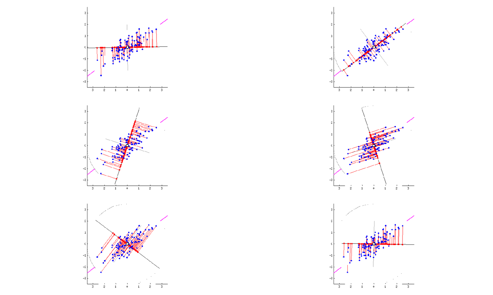
The figure below visually explains what PCA does. The blue dots are original data points in 2D. The red dots are projected data onto 1D rotating line. The red dotted line from blue points to red points are the trace of the projection. When the moving line overlaps with the pink line, the projected dot on the line is most widely distributed. If we apply PCA to this 2D data, 1D data can be obtained on this 1D line.

Visual Example of Dimensionality Reduction with PCA
Fig.1 PCA to project 2D data into 1D dimension from R-bloggers PCA in R

Reference

Describe An Array

Goal

This post aims to describe an array using pandas. As an example, Boston Housing Data is used in this post.

Reference

Libraries

In [13]:
import pandas as pd
from sklearn.datasets import load_boston
%matplotlib inline

Create an array

In [4]:
boston = load_boston()
df_boston = pd.DataFrame(boston['data'], columns=boston['feature_names'])
df_boston.head()
Out[4]:
CRIM ZN INDUS CHAS NOX RM AGE DIS RAD TAX PTRATIO B LSTAT
0 0.00632 18.0 2.31 0.0 0.538 6.575 65.2 4.0900 1.0 296.0 15.3 396.90 4.98
1 0.02731 0.0 7.07 0.0 0.469 6.421 78.9 4.9671 2.0 242.0 17.8 396.90 9.14
2 0.02729 0.0 7.07 0.0 0.469 7.185 61.1 4.9671 2.0 242.0 17.8 392.83 4.03
3 0.03237 0.0 2.18 0.0 0.458 6.998 45.8 6.0622 3.0 222.0 18.7 394.63 2.94
4 0.06905 0.0 2.18 0.0 0.458 7.147 54.2 6.0622 3.0 222.0 18.7 396.90 5.33

Describe numerical values

pandas DataFrame has a method, called describe, which shows basic statistics based on the data types for each columns

In [5]:
df_boston.describe()
Out[5]:
CRIM ZN INDUS CHAS NOX RM AGE DIS RAD TAX PTRATIO B LSTAT
count 506.000000 506.000000 506.000000 506.000000 506.000000 506.000000 506.000000 506.000000 506.000000 506.000000 506.000000 506.000000 506.000000
mean 3.613524 11.363636 11.136779 0.069170 0.554695 6.284634 68.574901 3.795043 9.549407 408.237154 18.455534 356.674032 12.653063
std 8.601545 23.322453 6.860353 0.253994 0.115878 0.702617 28.148861 2.105710 8.707259 168.537116 2.164946 91.294864 7.141062
min 0.006320 0.000000 0.460000 0.000000 0.385000 3.561000 2.900000 1.129600 1.000000 187.000000 12.600000 0.320000 1.730000
25% 0.082045 0.000000 5.190000 0.000000 0.449000 5.885500 45.025000 2.100175 4.000000 279.000000 17.400000 375.377500 6.950000
50% 0.256510 0.000000 9.690000 0.000000 0.538000 6.208500 77.500000 3.207450 5.000000 330.000000 19.050000 391.440000 11.360000
75% 3.677083 12.500000 18.100000 0.000000 0.624000 6.623500 94.075000 5.188425 24.000000 666.000000 20.200000 396.225000 16.955000
max 88.976200 100.000000 27.740000 1.000000 0.871000 8.780000 100.000000 12.126500 24.000000 711.000000 22.000000 396.900000 37.970000