Goal¶

This post aims to introduce how to conduct dimensionality reduction with Principal Component Analysis (PCA).

Dimensionality reduction with PCA can be used as a part of preprocessing to improve the accuracy of prediction when we have a lot of features that has correlation mutually.

The figure below visually explains what PCA does. The blue dots are original data points in 2D. The red dots are projected data onto 1D rotating line. The red dotted line from blue points to red points are the trace of the projection. When the moving line overlaps with the pink line, the projected dot on the line is most widely distributed. If we apply PCA to this 2D data, 1D data can be obtained on this 1D line.

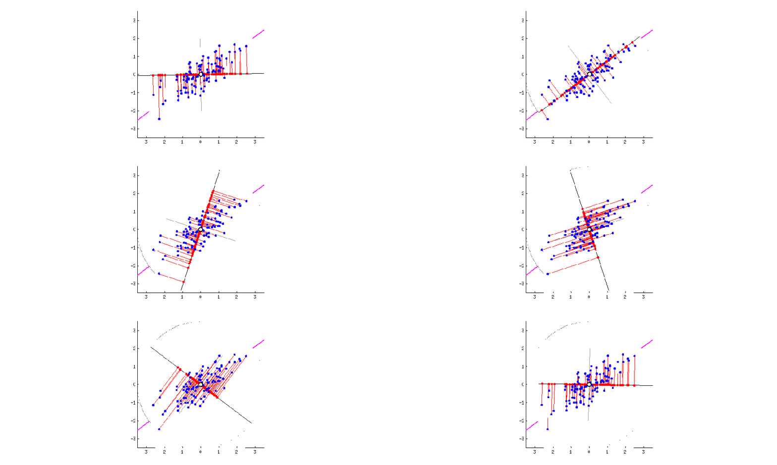
Visual Example of Dimensionality Reduction with PCA — Fig.1 PCA to project 2D data into 1D dimension from R-bloggers PCA in R

Reference

Libraries¶

In [40]:

import numpy as np
import pandas as pd
from sklearn.datasets import load_wine
from sklearn.decomposition import PCA
from sklearn.preprocessing import StandardScaler
from sklearn.pipeline import Pipeline
import matplotlib.pyplot as plt
%matplotlib inline

Create dataset¶

In [64]:

wine = load_wine()
df_wine = pd.DataFrame(wine['data'], columns=[wine['feature_names']])
print('df_wine.shape:', df_wine.shape)
df_wine.head()

df_wine.shape: (178, 13)

Out[64]:

	alcohol	malic_acid	ash	alcalinity_of_ash	magnesium	total_phenols	flavanoids	nonflavanoid_phenols	proanthocyanins	color_intensity	hue	od280/od315_of_diluted_wines	proline
0	14.23	1.71	2.43	15.6	127.0	2.80	3.06	0.28	2.29	5.64	1.04	3.92	1065.0
1	13.20	1.78	2.14	11.2	100.0	2.65	2.76	0.26	1.28	4.38	1.05	3.40	1050.0
2	13.16	2.36	2.67	18.6	101.0	2.80	3.24	0.30	2.81	5.68	1.03	3.17	1185.0
3	14.37	1.95	2.50	16.8	113.0	3.85	3.49	0.24	2.18	7.80	0.86	3.45	1480.0
4	13.24	2.59	2.87	21.0	118.0	2.80	2.69	0.39	1.82	4.32	1.04	2.93	735.0

Apply Normalization¶

Typically, normalization would be applied before PCA since one of the variable with larger numbers could be dominant to explain the variance.

In [44]:

scaler = StandardScaler()
df_wine_norm = pd.DataFrame(scaler.fit_transform(df_wine))
df_wine_norm.head()

Out[44]:

	0	1	2	3	4	5	6	7	8	9	10	11	12
0	1.518613	-0.562250	0.232053	-1.169593	1.913905	0.808997	1.034819	-0.659563	1.224884	0.251717	0.362177	1.847920	1.013009
1	0.246290	-0.499413	-0.827996	-2.490847	0.018145	0.568648	0.733629	-0.820719	-0.544721	-0.293321	0.406051	1.113449	0.965242
2	0.196879	0.021231	1.109334	-0.268738	0.088358	0.808997	1.215533	-0.498407	2.135968	0.269020	0.318304	0.788587	1.395148
3	1.691550	-0.346811	0.487926	-0.809251	0.930918	2.491446	1.466525	-0.981875	1.032155	1.186068	-0.427544	1.184071	2.334574
4	0.295700	0.227694	1.840403	0.451946	1.281985	0.808997	0.663351	0.226796	0.401404	-0.319276	0.362177	0.449601	-0.037874

In [47]:

# Mean is close to 0, and std is close to 1
df_wine_norm.describe()

Out[47]:

	0	1	2	3	4	5	6	7	8	9	10	11	12
count	1.780000e+02	1.780000e+02	1.780000e+02	1.780000e+02	1.780000e+02	1.780000e+02	1.780000e+02	1.780000e+02	1.780000e+02	1.780000e+02	1.780000e+02	1.780000e+02	1.780000e+02
mean	7.943708e-15	3.592632e-16	-4.066660e-15	-7.983626e-17	-7.983626e-17	-3.991813e-17	9.979533e-16	-5.588538e-16	-1.656602e-15	-3.442939e-16	1.636643e-15	2.235415e-15	-1.197544e-16
std	1.002821e+00	1.002821e+00	1.002821e+00	1.002821e+00	1.002821e+00	1.002821e+00	1.002821e+00	1.002821e+00	1.002821e+00	1.002821e+00	1.002821e+00	1.002821e+00	1.002821e+00
min	-2.434235e+00	-1.432983e+00	-3.679162e+00	-2.671018e+00	-2.088255e+00	-2.107246e+00	-1.695971e+00	-1.868234e+00	-2.069034e+00	-1.634288e+00	-2.094732e+00	-1.895054e+00	-1.493188e+00
25%	-7.882448e-01	-6.587486e-01	-5.721225e-01	-6.891372e-01	-8.244151e-01	-8.854682e-01	-8.275393e-01	-7.401412e-01	-5.972835e-01	-7.951025e-01	-7.675624e-01	-9.522483e-01	-7.846378e-01
50%	6.099988e-02	-4.231120e-01	-2.382132e-02	1.518295e-03	-1.222817e-01	9.595986e-02	1.061497e-01	-1.760948e-01	-6.289785e-02	-1.592246e-01	3.312687e-02	2.377348e-01	-2.337204e-01
75%	8.361286e-01	6.697929e-01	6.981085e-01	6.020883e-01	5.096384e-01	8.089974e-01	8.490851e-01	6.095413e-01	6.291754e-01	4.939560e-01	7.131644e-01	7.885875e-01	7.582494e-01
max	2.259772e+00	3.109192e+00	3.156325e+00	3.154511e+00	4.371372e+00	2.539515e+00	3.062832e+00	2.402403e+00	3.485073e+00	3.435432e+00	3.301694e+00	1.960915e+00	2.971473e+00

Apply PCA¶

In [63]:

pca = PCA()
df_wine_pca = pd.DataFrame(pca.fit_transform(df_wine_norm))
df_wine_pca.head()

Out[63]:

	0	1	2	3	4	5	6	7	8	9	10	11	12
0	3.316751	-1.443463	-0.165739	-0.215631	0.693043	-0.223880	0.596427	0.065139	0.641443	1.020956	-0.451563	0.540810	-0.066239
1	2.209465	0.333393	-2.026457	-0.291358	-0.257655	-0.927120	0.053776	1.024416	-0.308847	0.159701	-0.142657	0.388238	0.003637
2	2.516740	-1.031151	0.982819	0.724902	-0.251033	0.549276	0.424205	-0.344216	-1.177834	0.113361	-0.286673	0.000584	0.021717
3	3.757066	-2.756372	-0.176192	0.567983	-0.311842	0.114431	-0.383337	0.643593	0.052544	0.239413	0.759584	-0.242020	-0.369484
4	1.008908	-0.869831	2.026688	-0.409766	0.298458	-0.406520	0.444074	0.416700	0.326819	-0.078366	-0.525945	-0.216664	-0.079364

In [58]:

fig, axes = plt.subplots(1, 2, figsize=(9, 3))
axes[0].plot(pca.explained_variance_);
axes[0].set_title('Explained Variance')
axes[1].plot(np.cumsum(pca.explained_variance_ratio_));
axes[1].axhline(y=0.95, c='r', ls='-.')
axes[1].set_title('Cumulative Explained Variance Ratio')
plt.tight_layout()

Normalization & PCA together by `Pipeline`¶

In the below case, the number of principal component is automatically selected to 5.

In [62]:

pipeline = Pipeline([('scaling', StandardScaler()), ('pca', PCA(n_components=5))])
df_wine_pca_pipe = pd.DataFrame(pipeline.fit_transform(df_wine))
df_wine_pca_pipe.head()

Out[62]:

	0	1	2	3	4
0	3.316751	-1.443463	-0.165739	-0.215631	0.693043
1	2.209465	0.333393	-2.026457	-0.291358	-0.257655
2	2.516740	-1.031151	0.982819	0.724902	-0.251033
3	3.757066	-2.756372	-0.176192	0.567983	-0.311842
4	1.008908	-0.869831	2.026688	-0.409766	0.298458