Posts about PCA

Anomaly Detection by PCA in PyOD

Goal

This post aims to introduce how to detect anomaly using PCA in pyod.

image

Reference

Libraries

In [31]:
import pandas as pd
import numpy as np
import matplotlib.pyplot as plt
import seaborn as sns
%matplotlib inline

# PyOD
from pyod.utils.data import generate_data, get_outliers_inliers
from pyod.models.pca import PCA
from pyod.utils.data import evaluate_print
from pyod.utils.example import visualize

Create a data

In [66]:
X_train, y_train = generate_data(behaviour='new', n_features=5, train_only=True)
df_train = pd.DataFrame(X_train)
df_train['y'] = y_train
In [50]:
df_train.head()
Out[50]:
0 1 2 3 4 y
0 5.475324 4.882372 5.337351 5.376340 4.104947 0.0
1 5.244566 5.626358 5.356578 4.341500 4.856838 0.0
2 4.597031 5.787669 5.959738 5.823086 6.012408 0.0
3 4.637728 4.639901 5.400144 6.074926 4.627883 0.0
4 4.639908 4.667926 6.077212 5.012901 3.718718 0.0
In [57]:
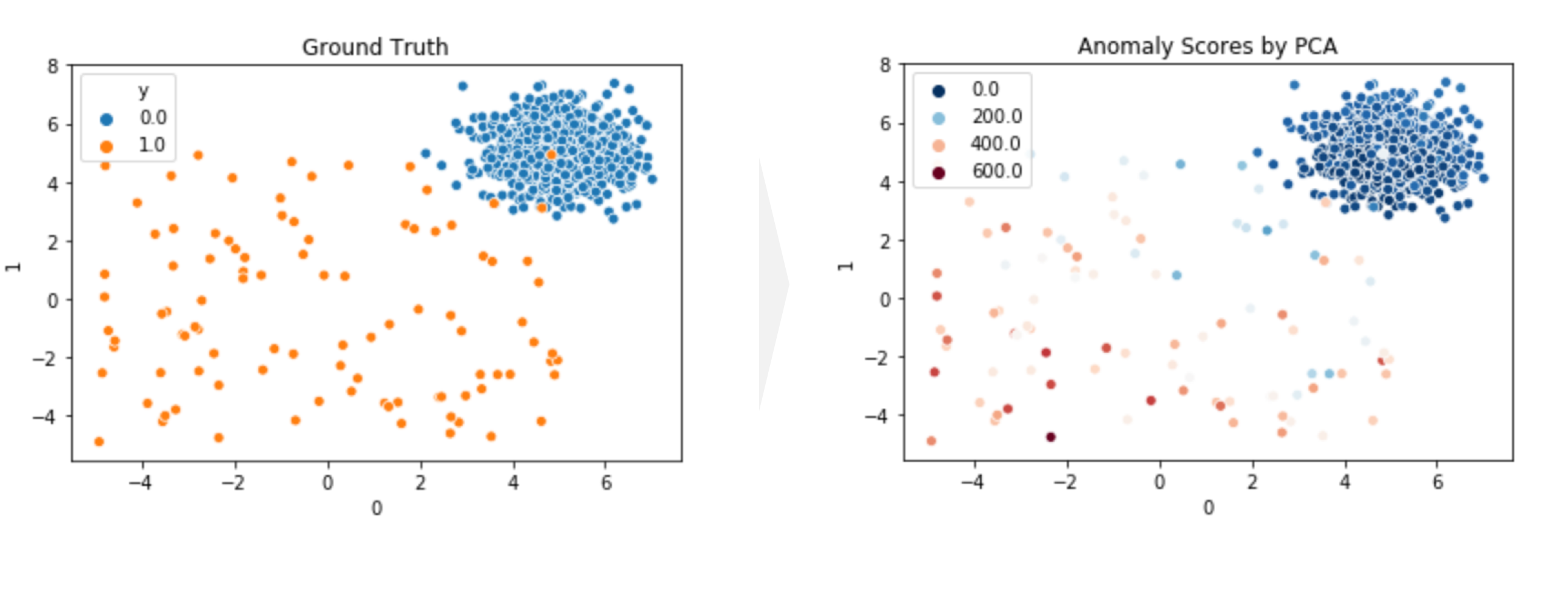
sns.scatterplot(x=0, y=1, hue='y', data=df_train);
plt.title('Ground Truth');

Train an unsupervised PCA

In [52]:
clf = PCA()
clf.fit(X_train)
Out[52]:
PCA(contamination=0.1, copy=True, iterated_power='auto', n_components=None,
  n_selected_components=None, random_state=None, standardization=True,
  svd_solver='auto', tol=0.0, weighted=True, whiten=False)

Evaluate training score

In [65]:
y_train_pred = clf.labels_
y_train_scores = clf.decision_scores_
sns.scatterplot(x=0, y=1, hue=y_train_scores, data=df_train, palette='RdBu_r');
plt.title('Anomaly Scores by PCA');

Dimensionality Reduction With PCA

Goal

This post aims to introduce how to conduct dimensionality reduction with Principal Component Analysis (PCA).

Dimensionality reduction with PCA can be used as a part of preprocessing to improve the accuracy of prediction when we have a lot of features that has correlation mutually.

The figure below visually explains what PCA does. The blue dots are original data points in 2D. The red dots are projected data onto 1D rotating line. The red dotted line from blue points to red points are the trace of the projection. When the moving line overlaps with the pink line, the projected dot on the line is most widely distributed. If we apply PCA to this 2D data, 1D data can be obtained on this 1D line.

Visual Example of Dimensionality Reduction with PCA
Fig.1 PCA to project 2D data into 1D dimension from R-bloggers PCA in R

Reference