Anomaly Detection by Auto Encoder (Deep Learning) in PyOD
Goal
This post aims to introduce how to detect anomaly using Auto Encoder (Deep Learning) in PyODand Keras / Tensorflow as backend.
This post aims to introduce how to detect anomaly using Auto Encoder (Deep Learning) in PyODand Keras / Tensorflow as backend.
import pandas as pd
import numpy as np
import matplotlib.pyplot as plt
import seaborn as sns
%matplotlib inline

# PyOD
from pyod.utils.data import generate_data, get_outliers_inliers
from pyod.models.pca import PCA
from pyod.utils.data import evaluate_print
from pyod.utils.example import visualize
X_train, y_train = generate_data(behaviour='new', n_features=5, train_only=True)
df_train = pd.DataFrame(X_train)
df_train['y'] = y_train
df_train.head()
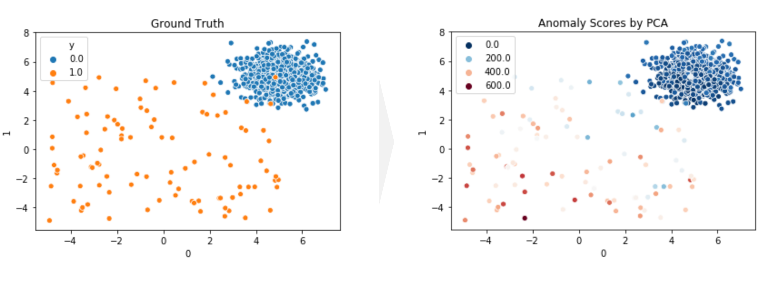
sns.scatterplot(x=0, y=1, hue='y', data=df_train);
plt.title('Ground Truth');

clf = PCA()
clf.fit(X_train)
y_train_pred = clf.labels_
y_train_scores = clf.decision_scores_
sns.scatterplot(x=0, y=1, hue=y_train_scores, data=df_train, palette='RdBu_r');
plt.title('Anomaly Scores by PCA');

This post aims to introduce how to make simulated data for anomaly detection using PyOD, which is outlier detection package.
Reference
import pandas as pd
import numpy as np
import matplotlib.pyplot as plt
%matplotlib inline

# PyOD
from pyod.utils.data import generate_data, get_outliers_inliers
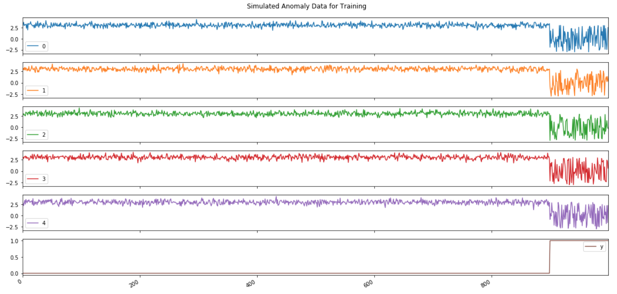
X_train, X_test, y_train, y_test = generate_data(behaviour='new', n_features=5)
df_tr = pd.DataFrame(X_train)
df_tr['y'] = y_train
df_te = pd.DataFrame(X_test)
df_te['y'] = y_test
df_tr.head()
axes = df_tr.plot(subplots=True, figsize=(16, 8), title='Simulated Anomaly Data for Training');
plt.tight_layout(rect=[0, 0.03, 1, 0.95])

axes = df_te.plot(subplots=True, figsize=(16, 8), title='Simulated Anomaly Data for Test');
plt.tight_layout(rect=[0, 0.03, 1, 0.95])