How to visualize a decision tree beyond scikit-learn

Goal

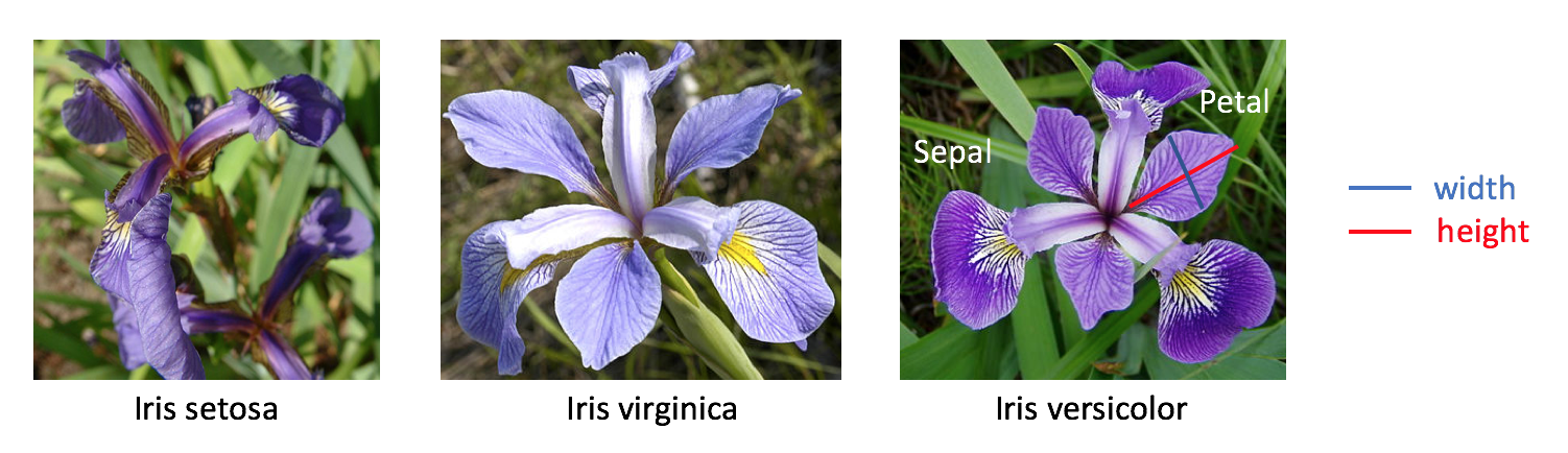
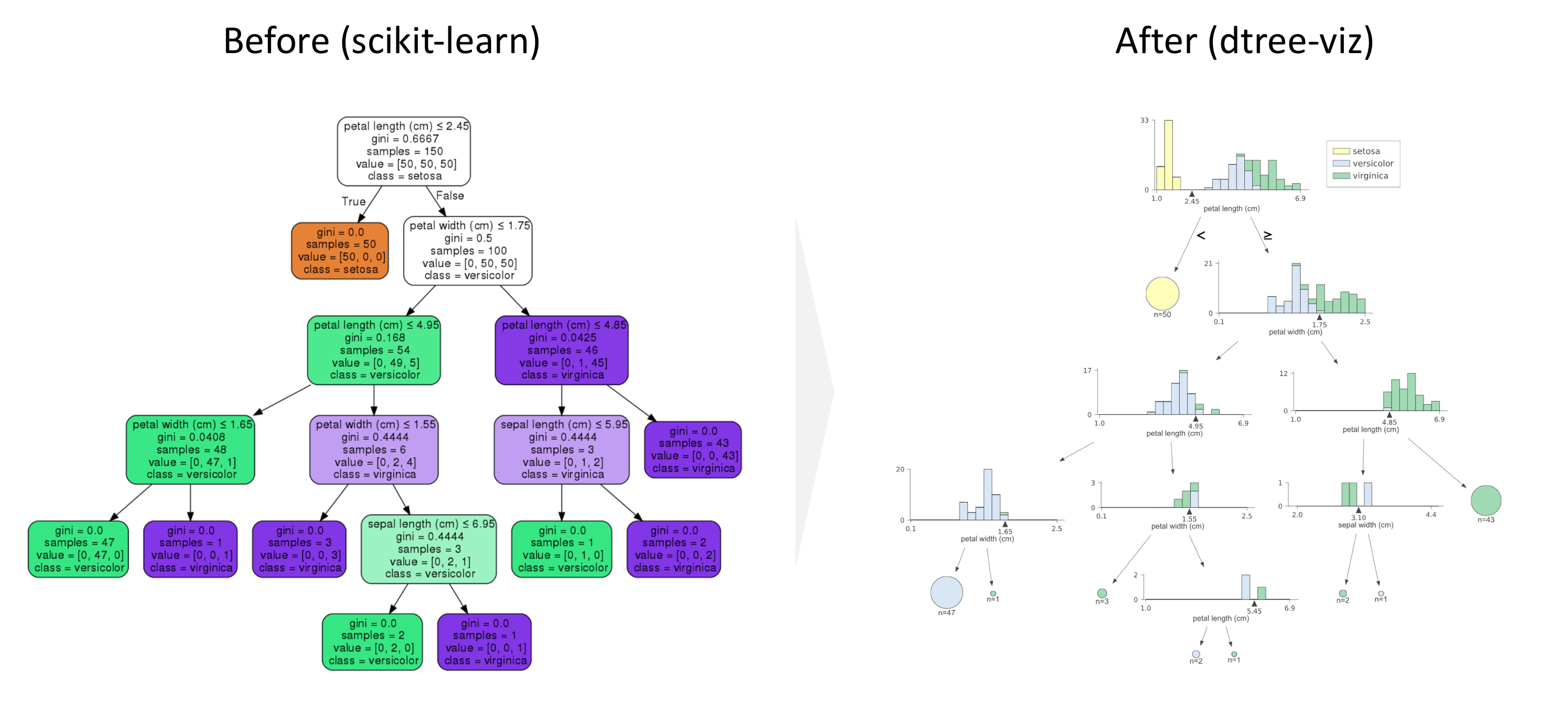
The goal in this post is to introduce dtreeviz to visualize a decision tree for classification more nicely than what scikit-learn can visualize. We will walk through the tutorial for decision trees in Scikit-learn using iris data set.

Note that if we use a decision tree for regression, the visualization would be different.

image

image

Pre-requisite

First of install the module using pip or conda command as below.

In [1]:
# !pip install dtreeviz
# ! pip install git+https://github.com/gautamkarnik/dtreeviz.git@update-for-cairo 
# as of Apr, 5, 2019 need to use this pull request on Mac OSX 10.13. this pull request will be merged soon 

Load Iris Dataset

In [2]:
import pandas as pd
import numpy as np
from sklearn.datasets import load_iris, load_boston
from sklearn import tree

iris = load_iris()
df_iris = pd.DataFrame(iris['data'], 
                       columns=iris['feature_names'])
df_iris['target'] = iris['target']
df_iris.head()
Out[2]:
sepal length (cm) sepal width (cm) petal length (cm) petal width (cm) target
0 5.1 3.5 1.4 0.2 0
1 4.9 3.0 1.4 0.2 0
2 4.7 3.2 1.3 0.2 0
3 4.6 3.1 1.5 0.2 0
4 5.0 3.6 1.4 0.2 0

Train a Decision tree

In [3]:
# Train the Decision tree model
clf = tree.DecisionTreeClassifier()
clf = clf.fit(iris.data, iris.target)

Visualize a Decision Tree

Scikit-learn

In [4]:
import graphviz 
dot_data = tree.export_graphviz(clf, out_file=None, 
                     feature_names=iris.feature_names,  
                     class_names=iris.target_names,  
                     filled=True, rounded=True,  
                     special_characters=True)  

graph = graphviz.Source(dot_data)  
graph 
Out[4]:
Tree 0 petal length (cm) ≤ 2.45gini = 0.667samples = 150value = [50, 50, 50]class = setosa1 gini = 0.0samples = 50value = [50, 0, 0]class = setosa0->1 True2 petal width (cm) ≤ 1.75gini = 0.5samples = 100value = [0, 50, 50]class = versicolor0->2 False3 petal length (cm) ≤ 4.95gini = 0.168samples = 54value = [0, 49, 5]class = versicolor2->3 12 petal length (cm) ≤ 4.85gini = 0.043samples = 46value = [0, 1, 45]class = virginica2->12 4 petal width (cm) ≤ 1.65gini = 0.041samples = 48value = [0, 47, 1]class = versicolor3->4 7 petal width (cm) ≤ 1.55gini = 0.444samples = 6value = [0, 2, 4]class = virginica3->7 5 gini = 0.0samples = 47value = [0, 47, 0]class = versicolor4->5 6 gini = 0.0samples = 1value = [0, 0, 1]class = virginica4->6 8 gini = 0.0samples = 3value = [0, 0, 3]class = virginica7->8 9 petal length (cm) ≤ 5.45gini = 0.444samples = 3value = [0, 2, 1]class = versicolor7->9 10 gini = 0.0samples = 2value = [0, 2, 0]class = versicolor9->10 11 gini = 0.0samples = 1value = [0, 0, 1]class = virginica9->11 13 sepal width (cm) ≤ 3.1gini = 0.444samples = 3value = [0, 1, 2]class = virginica12->13 16 gini = 0.0samples = 43value = [0, 0, 43]class = virginica12->16 14 gini = 0.0samples = 2value = [0, 0, 2]class = virginica13->14 15 gini = 0.0samples = 1value = [0, 1, 0]class = versicolor13->15

dtreeviz

In [5]:
from dtreeviz.trees import dtreeviz
viz = dtreeviz(clf,
               iris['data'],
               iris['target'],
               target_name='',
               feature_names=np.array(iris['feature_names']),
               class_names={0:'setosa',1:'versicolor',2:'virginica'})
              
viz
Out[5]:
G cluster_legendnode4 node7 leaf5 node4->leaf5 leaf6 node4->leaf6 node9 leaf10 node9->leaf10 leaf11 node9->leaf11 node7->node9 leaf8 node7->leaf8 node3 node3->node4 node3->node7 node12 node13 leaf14 node13->leaf14 leaf15 node13->leaf15 leaf16 node12->node13 node12->leaf16 node2 node2->node3 node2->node12 node0 node0->node2 leaf1 node0->leaf1 <legend

What is better for drtreeviz

  • You can see the distribution for each class at each node
  • You can see where is the decision boundary for each split
  • You can see the sample sie at each leaf as the size of the circle

Comments

Comments powered by Disqus