Calculate The Determinant Of A Matrix

Goal

This post aims to show how to calculate the determinant of a matrix using numpy i.e., $|A|$

For example, if we have

$$A = \begin{bmatrix} a & b \\ c & d \end{bmatrix} $$

Then, $|A|$ is defined as

$$|A| = \begin{vmatrix} a & b \\ c & d \end{vmatrix} = ab - bc $$

Reference:

Libraries

In [3]:
import numpy as np

Create a matrix

In [6]:
a = np.array([[1,2], [3,4]]) 
a
Out[6]:
array([[1, 2],
       [3, 4]])

Calculate the determinant

In [7]:
print(np.linalg.det(a))
-2.0000000000000004
In [8]:
a[0, 0] * a[1, 1] - a[0, 1] * a[1, 0]
Out[8]:
-2

Dimensionality Reduction With PCA

Goal

This post aims to introduce how to conduct dimensionality reduction with Principal Component Analysis (PCA).

Dimensionality reduction with PCA can be used as a part of preprocessing to improve the accuracy of prediction when we have a lot of features that has correlation mutually.

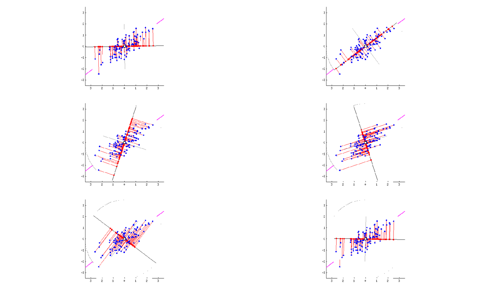
The figure below visually explains what PCA does. The blue dots are original data points in 2D. The red dots are projected data onto 1D rotating line. The red dotted line from blue points to red points are the trace of the projection. When the moving line overlaps with the pink line, the projected dot on the line is most widely distributed. If we apply PCA to this 2D data, 1D data can be obtained on this 1D line.

Visual Example of Dimensionality Reduction with PCA
Fig.1 PCA to project 2D data into 1D dimension from R-bloggers PCA in R

Reference

Describe An Array

Goal

This post aims to describe an array using pandas. As an example, Boston Housing Data is used in this post.

Reference

Libraries

In [13]:
import pandas as pd
from sklearn.datasets import load_boston
%matplotlib inline

Create an array

In [4]:
boston = load_boston()
df_boston = pd.DataFrame(boston['data'], columns=boston['feature_names'])
df_boston.head()
Out[4]:
CRIM ZN INDUS CHAS NOX RM AGE DIS RAD TAX PTRATIO B LSTAT
0 0.00632 18.0 2.31 0.0 0.538 6.575 65.2 4.0900 1.0 296.0 15.3 396.90 4.98
1 0.02731 0.0 7.07 0.0 0.469 6.421 78.9 4.9671 2.0 242.0 17.8 396.90 9.14
2 0.02729 0.0 7.07 0.0 0.469 7.185 61.1 4.9671 2.0 242.0 17.8 392.83 4.03
3 0.03237 0.0 2.18 0.0 0.458 6.998 45.8 6.0622 3.0 222.0 18.7 394.63 2.94
4 0.06905 0.0 2.18 0.0 0.458 7.147 54.2 6.0622 3.0 222.0 18.7 396.90 5.33

Describe numerical values

pandas DataFrame has a method, called describe, which shows basic statistics based on the data types for each columns

In [5]:
df_boston.describe()
Out[5]:
CRIM ZN INDUS CHAS NOX RM AGE DIS RAD TAX PTRATIO B LSTAT
count 506.000000 506.000000 506.000000 506.000000 506.000000 506.000000 506.000000 506.000000 506.000000 506.000000 506.000000 506.000000 506.000000
mean 3.613524 11.363636 11.136779 0.069170 0.554695 6.284634 68.574901 3.795043 9.549407 408.237154 18.455534 356.674032 12.653063
std 8.601545 23.322453 6.860353 0.253994 0.115878 0.702617 28.148861 2.105710 8.707259 168.537116 2.164946 91.294864 7.141062
min 0.006320 0.000000 0.460000 0.000000 0.385000 3.561000 2.900000 1.129600 1.000000 187.000000 12.600000 0.320000 1.730000
25% 0.082045 0.000000 5.190000 0.000000 0.449000 5.885500 45.025000 2.100175 4.000000 279.000000 17.400000 375.377500 6.950000
50% 0.256510 0.000000 9.690000 0.000000 0.538000 6.208500 77.500000 3.207450 5.000000 330.000000 19.050000 391.440000 11.360000
75% 3.677083 12.500000 18.100000 0.000000 0.624000 6.623500 94.075000 5.188425 24.000000 666.000000 20.200000 396.225000 16.955000
max 88.976200 100.000000 27.740000 1.000000 0.871000 8.780000 100.000000 12.126500 24.000000 711.000000 22.000000 396.900000 37.970000

Random Forest Classifer

Goal

This post aims to introduce how to train random forest classifier, which is one of most popular machine learning model.

Reference

Libraries

In [12]:
import pandas as pd
import numpy as np
from sklearn.datasets import make_blobs
from sklearn.model_selection import cross_val_score
from sklearn.ensemble import RandomForestClassifier
import matplotlib.pyplot as plt
%matplotlib inline

Load Data

In [6]:
X, y = make_blobs(n_samples=10000, n_features=10, centers=100, random_state=0)
df_X = pd.DataFrame(X)
df_X.head()
Out[6]:
0 1 2 3 4 5 6 7 8 9
0 6.469076 4.250703 -8.636944 4.044785 9.017254 4.535872 -4.670276 -0.481728 -6.449961 -2.659850
1 6.488564 9.379570 10.327917 -1.765055 -2.068842 -9.537790 3.936380 3.375421 7.412737 -9.722844
2 8.373928 -10.143423 -3.527536 -7.338834 1.385557 6.961417 -4.504456 -7.315360 -2.330709 6.440872
3 -3.414101 -2.019790 -2.748108 4.168691 -5.788652 -7.468685 -1.719800 -5.302655 4.534099 -4.613695
4 -1.330023 -3.725465 9.559999 -6.751356 -7.407864 -2.131515 1.766013 2.381506 -1.886568 8.667311
In [8]:
df_y = pd.DataFrame(y, columns=['y'])
df_y.head()
Out[8]:
y
0 85
1 64
2 93
3 46
4 61

Train a model using Cross Validation

In [19]:
clf = RandomForestClassifier(n_estimators=10, max_depth=None, min_samples_split=2, random_state=0)
scores = cross_val_score(clf, X, y, cv=5, verbose=1)
scores.mean()                               
[Parallel(n_jobs=1)]: Using backend SequentialBackend with 1 concurrent workers.
[Parallel(n_jobs=1)]: Done   5 out of   5 | elapsed:    1.8s finished
Out[19]:
0.9997
In [15]:
pd.DataFrame(scores, columns=['CV Scores']).plot();

Histograms In Pandas

Goal

This post aims to introduce how to create histogram plot using pandas

Libraries

In [3]:
import pandas as pd
import numpy as np
import matplotlib.pyplot as plt
%matplotlib inline

Create data

In [4]:
df = pd.DataFrame(np.random.random(100))
df.head()
Out[4]:
0
0 0.984265
1 0.862053
2 0.360947
3 0.146953
4 0.439591

Create Histogram

In [11]:
df.plot(kind='hist', bins=50);

Loading scikit-learn's Boston Housing Dataset

Goal

This post aims to introduce how to load Boston housing using scikit-learn

Library

In [8]:
from sklearn.datasets import load_boston
import pandas as pd

Load Dataset

In [3]:
boston = load_boston()
In [4]:
type(boston)
Out[4]:
sklearn.utils.Bunch
In [6]:
boston.keys()
Out[6]:
dict_keys(['data', 'target', 'feature_names', 'DESCR', 'filename'])

Data

In [9]:
pd.DataFrame(boston.data).head()
Out[9]:
0 1 2 3 4 5 6 7 8 9 10 11 12
0 0.00632 18.0 2.31 0.0 0.538 6.575 65.2 4.0900 1.0 296.0 15.3 396.90 4.98
1 0.02731 0.0 7.07 0.0 0.469 6.421 78.9 4.9671 2.0 242.0 17.8 396.90 9.14
2 0.02729 0.0 7.07 0.0 0.469 7.185 61.1 4.9671 2.0 242.0 17.8 392.83 4.03
3 0.03237 0.0 2.18 0.0 0.458 6.998 45.8 6.0622 3.0 222.0 18.7 394.63 2.94
4 0.06905 0.0 2.18 0.0 0.458 7.147 54.2 6.0622 3.0 222.0 18.7 396.90 5.33

Target

In [12]:
pd.DataFrame(boston.target).head()
Out[12]:
0
0 24.0
1 21.6
2 34.7
3 33.4
4 36.2

Feature Name

In [17]:
print(boston.feature_names)
['CRIM' 'ZN' 'INDUS' 'CHAS' 'NOX' 'RM' 'AGE' 'DIS' 'RAD' 'TAX' 'PTRATIO'
 'B' 'LSTAT']

Description

In [19]:
print(boston.DESCR)
.. _boston_dataset:

Boston house prices dataset
---------------------------

**Data Set Characteristics:**  

    :Number of Instances: 506 

    :Number of Attributes: 13 numeric/categorical predictive. Median Value (attribute 14) is usually the target.

    :Attribute Information (in order):
        - CRIM     per capita crime rate by town
        - ZN       proportion of residential land zoned for lots over 25,000 sq.ft.
        - INDUS    proportion of non-retail business acres per town
        - CHAS     Charles River dummy variable (= 1 if tract bounds river; 0 otherwise)
        - NOX      nitric oxides concentration (parts per 10 million)
        - RM       average number of rooms per dwelling
        - AGE      proportion of owner-occupied units built prior to 1940
        - DIS      weighted distances to five Boston employment centres
        - RAD      index of accessibility to radial highways
        - TAX      full-value property-tax rate per $10,000
        - PTRATIO  pupil-teacher ratio by town
        - B        1000(Bk - 0.63)^2 where Bk is the proportion of blacks by town
        - LSTAT    % lower status of the population
        - MEDV     Median value of owner-occupied homes in $1000's

    :Missing Attribute Values: None

    :Creator: Harrison, D. and Rubinfeld, D.L.

This is a copy of UCI ML housing dataset.
https://archive.ics.uci.edu/ml/machine-learning-databases/housing/


This dataset was taken from the StatLib library which is maintained at Carnegie Mellon University.

The Boston house-price data of Harrison, D. and Rubinfeld, D.L. 'Hedonic
prices and the demand for clean air', J. Environ. Economics & Management,
vol.5, 81-102, 1978.   Used in Belsley, Kuh & Welsch, 'Regression diagnostics
...', Wiley, 1980.   N.B. Various transformations are used in the table on
pages 244-261 of the latter.

The Boston house-price data has been used in many machine learning papers that address regression
problems.   
     
.. topic:: References

   - Belsley, Kuh & Welsch, 'Regression diagnostics: Identifying Influential Data and Sources of Collinearity', Wiley, 1980. 244-261.
   - Quinlan,R. (1993). Combining Instance-Based and Model-Based Learning. In Proceedings on the Tenth International Conference of Machine Learning, 236-243, University of Massachusetts, Amherst. Morgan Kaufmann.
1039. Minimum Score Triangulation of Polygon

Problem Setting

Given N, consider a convex N-sided polygon with vertices labelled A[0], A[i], ..., A[N-1] in clockwise order.

Suppose you triangulate the polygon into N-2 triangles. For each triangle, the value of that triangle is the product of the labels of the vertices, and the total score of the triangulation is the sum of these values over all N-2 triangles in the triangulation.

Return the smallest possible total score that you can achieve with some triangulation of the polygon.

Source: LeetCode link

image

The solution is based on dynamic programming like below. This gif is explained in the last part.

2019-05-10_1039_dp_image1