Goal¶

This post aims to introduce how to explain the interaction values for the model's prediction by SHAP. In this post, we will use data NHANES I (1971-1974) from National Health and Nutrition Examaination Survey.

Reference

Libraries¶

In [1]:

import shap
import xgboost
from sklearn.model_selection import train_test_split
import matplotlib.pyplot as plt
%matplotlib inline

Configuration¶

In [8]:

test_size = 0.2
random_state = 1

Load data for NHANES I¶

In [5]:

X, y = shap.datasets.nhanesi()
X.head()

Out[5]:

	Unnamed: 0	Age	Diastolic BP	Poverty index	Race	Red blood cells	Sedimentation rate	Serum Albumin	Serum Cholesterol	Serum Iron	Serum Magnesium	Serum Protein	Sex	Systolic BP	TIBC	TS	White blood cells	BMI	Pulse pressure
0	0	35.0	92.0	126.0	2.0	77.7	12.0	5.0	165.0	135.0	1.37	7.6	2.0	142.0	323.0	41.8	5.8	31.109434	50.0
1	1	71.0	78.0	210.0	2.0	77.7	37.0	4.0	298.0	89.0	1.38	6.4	2.0	156.0	331.0	26.9	5.3	32.362572	78.0
2	2	74.0	86.0	999.0	2.0	77.7	31.0	3.8	222.0	115.0	1.37	7.4	2.0	170.0	299.0	38.5	8.1	25.388497	84.0
3	3	64.0	92.0	385.0	1.0	77.7	30.0	4.3	265.0	94.0	1.97	7.3	2.0	172.0	349.0	26.9	6.7	26.446610	80.0
4	4	32.0	70.0	183.0	2.0	77.7	18.0	5.0	203.0	192.0	1.35	7.3	1.0	128.0	386.0	49.7	8.1	20.354684	58.0

In [7]:

y[:5]

Out[7]:

array([ 15.27465753,  11.58607306,   8.14908676, -21.09429224,
        -0.        ])

Split the data into training and test¶

In [9]:

X_train, X_test, y_train, y_test = train_test_split(
    X, y, test_size=test_size, random_state=random_state)

xgb_train = xgboost.DMatrix(X_train, label=y_train)
xgb_test = xgboost.DMatrix(X_test, label=y_test)

Create a XGBoost model¶

Model Configuration¶

In [10]:

# For Training
params_train = {
    "eta": 0.002,
    "max_depth": 3,
    "objective": "survival:cox",
    "subsample": 0.5
}

Train a model¶

In [11]:

model_train = xgboost.train(params_train, xgb_train, 
                            num_boost_round=10000, 
                            evals=[(xgb_test, "test")], 
                            verbose_eval=1000)

[0]	test-cox-nloglik:7.2544
[1000]	test-cox-nloglik:6.59596
[2000]	test-cox-nloglik:6.5461
[3000]	test-cox-nloglik:6.54169
[4000]	test-cox-nloglik:6.54415
[5000]	test-cox-nloglik:6.54855
[6000]	test-cox-nloglik:6.55272
[7000]	test-cox-nloglik:6.55845
[8000]	test-cox-nloglik:6.5622
[9000]	test-cox-nloglik:6.56736
[9999]	test-cox-nloglik:6.57163

Create an explainer¶

In [14]:

explainer = shap.TreeExplainer(model_train)
shap_values = explainer.shap_values(X_test)

Compute shap interaction values¶

In [17]:

shap_interaction_values = explainer.shap_interaction_values(X_test.iloc[:1000, :])

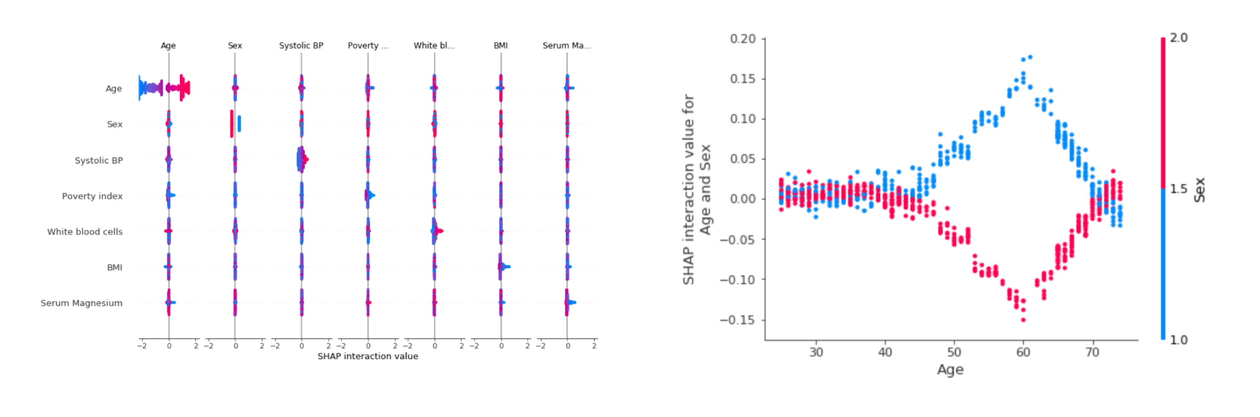
Interaction Values across variables¶

In [18]:

shap.summary_plot(shap_interaction_values, X_test.iloc[:1000,:])

Interaction Value Dependence¶

In [19]:

shap.dependence_plot(
    ("Age", "Sex"),
    shap_interaction_values, X_test.iloc[:1000,:],
    display_features=X_test.iloc[:1000,:]
)